FLARE User Guide

FLARE Users Guide and Tutorial

4/23/2020

Background
Requirements
1: Set up
2: Configure simulation (GLM)
3: Run your first simulation (GLM)
4: Examining FLARE output
5: Running GLM-AED
6: Modifying FLARE
7: Modifying FLARE for a new lake
Appendix: FLARE Configurations

Background

This document serves as a users guide and a tutorial for the FLARE (Forecasting Lake and Reservior Ecosystems) system (Thomas et al. 2020). FLARE generates forecasts and forecast uncertainty of water temperature and water quality for a 16-day time horizon at multiple depths of a lake or reservior. It uses data assimilation to update the initial starting point for a forecast and the model parameters based a real-time statistical comparsions to observations. While it has been developed, tested, and evaluated for Falling Creek Reservior in Vinton,VA (Thomas et al. 2020), this document provides guidance for adapting FLARE to different waterbodies.

FLARE is a set of R scripts that

• Downloads, cleans, organizes data required for data assimilation and forecasting
• Generating the inputs and configuration files required by the General Lake Model (GLM)
• Applying data assimilation to GLM
• Processing and archiving forecast output
• Visualizing forecast ouptut

FLARE uses the 1-D General Lake Model (Hipsey et al. 2019) as the mechanistic process model that predicts hydrodynamics of the lake or reservior. For forecasts of water quality, it uses GLM with the Aquatic Ecosystem Dynamics library. The binaries for GLM and GLM-AED are included in the FLARE code that is avialable on GitHub. FLARE requires GLM version 3.1 or higher.

More information about the GLM can be found here:

• GLM users guide
• GLM 3.0.0 manuscript
• GLM on GitHub
• AED on GitHub

FLARE development has been supported by grants from National Science Foundation (CNS-1737424, DEB-1753639, EF-1702506, DBI-1933016, DEB-1926050)

Requirements

• RStudio
• R packages
  • Tidyverse
    • uses tidyr version 1.0.0 or higher (uses pivot_longer and pivot_wider)
  • mvtnorm
  • ncdf4
  • testit
  • imputeTS
  • tools
  • rMR

1: Set up

To set up the files needed for FLARE perform either Step 1a or Step 1b

• Step 1a is the quickest way to get FLARE set-up but won’t have the most recent data or code.
• Step 1b is required if you want to automatically pull new data from GitHub
• Step 1c is uses a docker container that already has the libraries that FLARE requires installed. Similar to step 1a, the Docker container won’t have the most recent data or code.

1a: Pre-packaged code and data

Download and unzip the file here:

https://www.dropbox.com/s/enl9srn5rx7ecxp/flare_users_guide_files.zip?dl=0

1b: Generating directories, downloading code, and downloading data manually

Download FLARE code

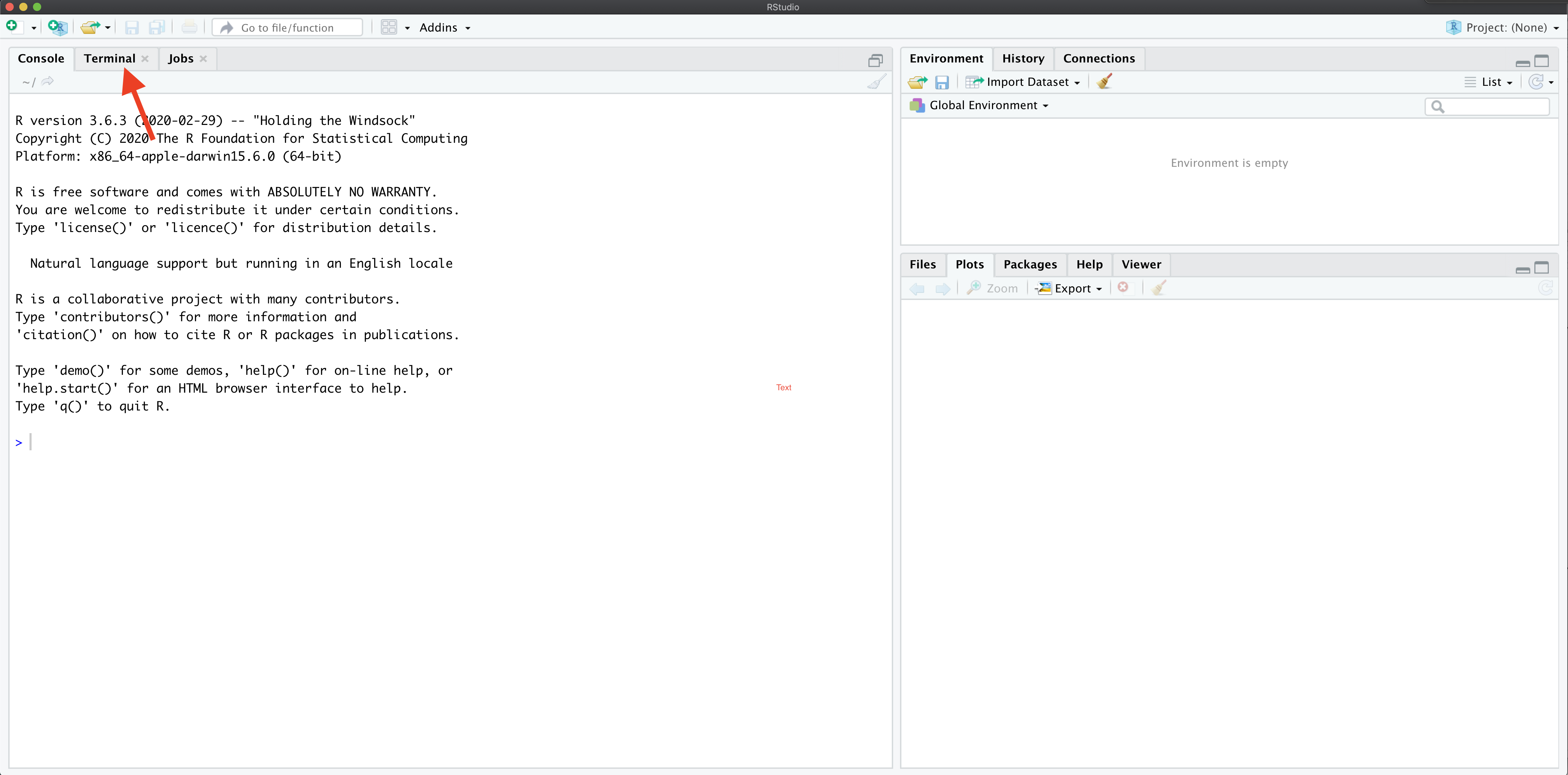
• Open R Studio

• Locate the terminal tab

• In the terminal, create the location on your computer where you want to save files for the tutorial using the command mkdir. For example:

  mkdir /Users/quinn/Dropbox/Research/SSC_forecasting/flare_training

  This will be called your tutorial directory below

• In the terminal, move to the new directory using the command cd. For example:

  cd /Users/quinn/Dropbox/Research/SSC_forecasting/flare_training

• In the terminal tab run the following command to download the FLARE code from Github

  git clone https://github.com/CareyLabVT/FLARE.git

  After the cloning process finishes, you should see a new folder named FLARE in your working directory

Download data

• Create a new directory for data used by FLARE in the tutorial directory. First, change your current directory to the tutorial directory using cd from the terminal tab (if you just ran the step above, you should already be in this directory). For example:

  cd /Users/quinn/Dropbox/Research/SSC_forecasting/flare_training

• Then, run the following line to create the directory:

  mkdir SCC_data

• Change your directory to this new data directory using cd

  cd SCC_data

• Download the met station data by running the following command in the terminal (this may take a while)

  git clone -b carina-data --single-branch https://github.com/CareyLabVT/SCCData.git carina-data

• Download the NOAA forecasts for FCR by running the following command in the terminal

  git clone -b fcre --single-branch https://github.com/CareyLabVT/noaa_gefs_forecasts.git fcre

• Download the catwalk data by running the following command in the terminal

  git clone -b mia-data --single-branch https://github.com/CareyLabVT/SCCData.git mia-data

• Download the weir data by running the following command in the terminal

  git clone -b diana-data --single-branch https://github.com/CareyLabVT/SCCData.git diana-data

• Download noaa forecasts by running the following command in the terminal

  git clone -b fcre --single-branch https://github.com/CareyLabVT/noaa_gefs_forecasts.git fcre

• Download non-sensor data by running the following command in the terminal

  git clone -b manual-data --single-branch https://github.com/CareyLabVT/SCCData.git manual-data

  The non-sensor data include

  • CTD data from EDI
  • SSS files
  • Nutrient chemistry from EDI
  • Weir data from EDI

• Download the met station from EDI (this file is too big for Github so you have to get it directory from EDI)

  • If you would like to do this manually, the file can be found at: https://portal.edirepository.org/nis/mapbrowse?packageid=edi.389.4. Download the file Met_final_2015_2019.csv and move it to your SCC_data/manual-data directory

Create directory for running FLARE

• Create a directory in your working directory (flare_training, not the SCC_data directory) using mkdir. For example:

  mkdir /Users/quinn/Dropbox/Research/SSC_forecasting/flare_training/flare_simulation

Copy the following files from FLARE/example_configuration_files to flare_simulation

• initiate_forecast_example.R
• glm3_woAED.nml
• configure_FLARE.R

1c: Using a Docker Container

Below are the steps for running FLARE as a Docker Container. If you already have Docker Desktop on your computer you can skip the first step.

• Download and install Docker Desktop from Docker.com
  • https://www.docker.com/products/docker-desktop
• Open a Terminal window in Mac or Command Prompt window in Windows
• Run this command in Terminal or Command Prompt (this will take a while to download) docker run --name flare-dev -e PASSWORD=password -p 8787:8787 flareforecast/flare_scc_tutorial2
• Open a webbrower and enter the following address: http://localhost:8787
• Enter the following user name and password
  • user: rstudio
  • password: password

2: Configure simulation (GLM)

A FLARE simulation with AED requires three files that should be in your flare_simulation directory (coppied to this location in the step above). The configuration funcations are spread across the files. These files are described in more detail below

• initiate_forecast_example.R
• glm3_woAED.nml
• configure_FLARE.R

initiate_forecast_example.R

This file is the main script that launches the FLARE code and plots the output. In this tutorial you will modify the following variables (for now only modify the first three as specified)

• data_location: This is the SCC_data directory (full path; you will need to change this to reflect the location of your directory)
• code_folder: This is the FLARE directory (full path; you will need to change this to reflect the location of your directory)
• forecast_location: This is the flare_simulation directory (full path; you will need to change this to reflect the location of your directory)
• execute_location: This is the same as forecast_location unless you are executing the simulation in a different directory. I use this to execute the code on a RAM disk to save read-writes to my hard disk. You don’t need to do this in the tutorial
• restart_file: This is the full path to the file that you want to use as initial conditions for the simulation. You will set this to NA if the simulation is not a continuation of a previous simulation.
• sim_name: a string with the name of your simulation. This will appear in your output file names
• forecast_days: This is your forecast horizon. The max is 16 days. Set to 0if only doing data assimilation with observed drivers.
• spin_up_days: set to zero. Don’t worry about this one.
• start_day_local: The date that your simulation starts. Uses the YYYY-MM-DD format (e.g., “2019-09-20”). 2018-07-12 is the first day in the SCC project (when the catwalk temperature data comes online)
• start_time_local: The time of day you want to start a forecast. Because GLM is a daily timestep model, the simulation will start at this time. It uses mm:hh:ss format and must only be a whole hour. It is in the local time zone of the lake in standard time. It can be any hour if only doing data assimilation with observed drivers (forecast_days = 0). If forecasting (forecast_days > 0) it is required to match up with the availability of a NOAA forecast. NOAA forecasts are available at the following times GMT so you must select a local time that matches one of these times (i.e., 07:00:00 at FCR is the 12:00:00 GMT NOAA forecast).
  • 00:00:00 GMT
  • 06:00:00 GMT
  • 12:00:00 GMT
  • 18:00:00 GMT
• forecast_start_day_local: The date that you want forecasting to start in your simulation. Uses the YYYY-MM-DD format (e.g., “2019-09-20”). The difference between start_time_local and forecast_start_day_local determines how many days of data assimilation occur using observed drivers before handing off to forecasted drivers and not assimilating data
• forecast_sss_on: Only used in AED simulations for setting the SSS (hypolimnetic oxygenation system) to on in the forecast

initiate_forecast_example.R loads Rscripts and runs the FLARE code with the EnKF function run_flare and the plotting code plot_forecast.

glm3_woAED.nml

glm3_woAED.nml is the configuration file that is required by GLM. It can be configurated to run only GLM or GLM + AED. This version is already configured to run only GLM for FCR and you do not need to modify it for the example simulation.

configure_FLARE.R

configure_FLARE.R has the bulk of the configurations for FLARE that you will set once and reuse (unlike initiate_forecast_example.R which changes when you want to forecast a new time period). The end of this document describes all of the configurations in configure_FLARE.R. Later in the tutorial, you will modify key configurations in configure_FLARE.R

If you set up your directories and modified the initiate_forecast_example.R as described above, then you will not need to modify configure_FLARE.R to do a test simulation.

3: Run your first simulation (GLM)

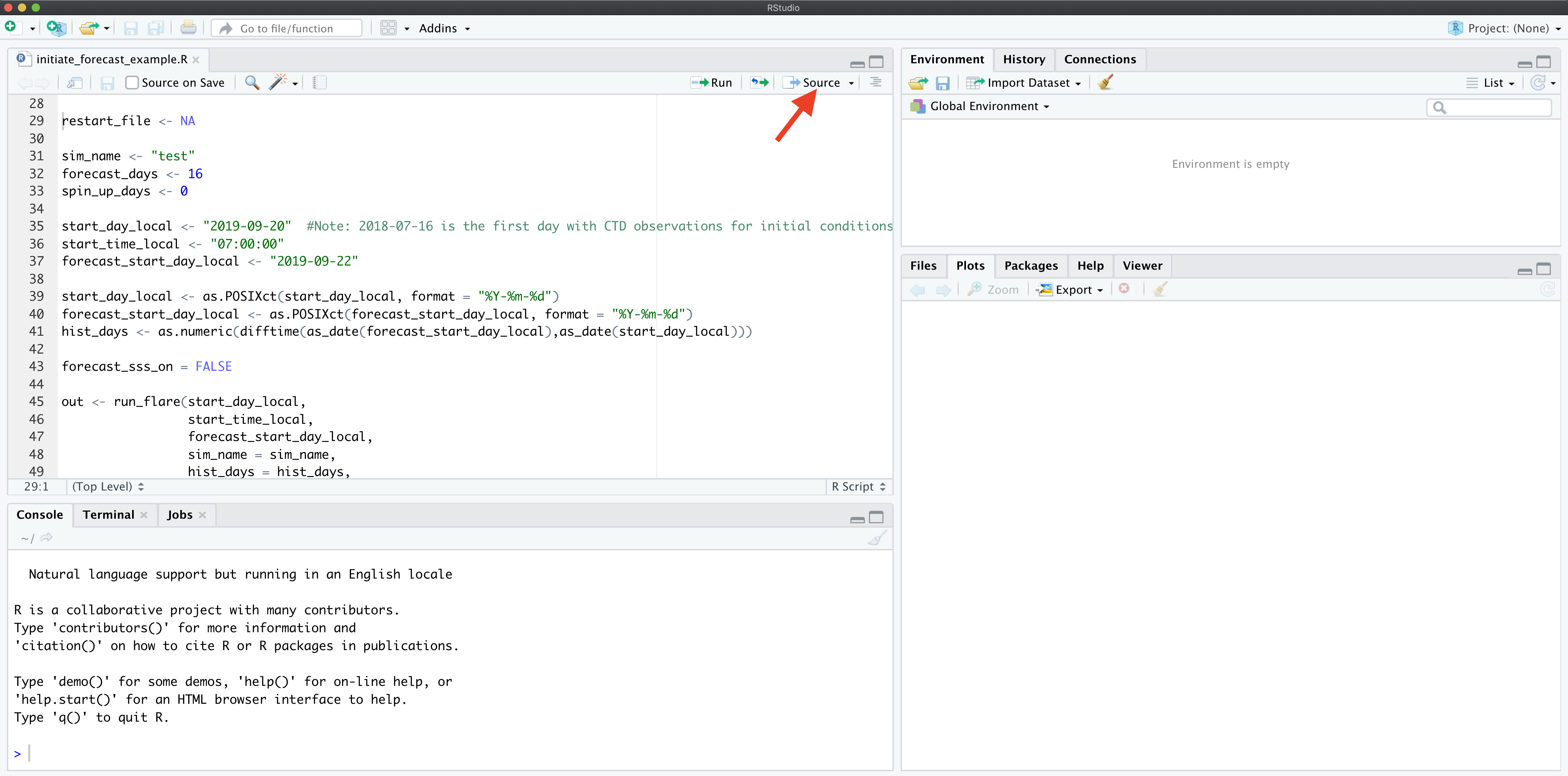
To run your first FLARE simulation confirm that the following variables are set in your initiate_forecast_example.R file:

• restart_file <- NA
• sim_name <- "test"
• forecast_days <- 16
• start_day_local <- "2018-07-12"
• start_time_local <- "07:00:00"
• forecast_start_day_local <- "2018-07-15"

Now source initiate_forecast_example.R.

You will find that a working_directory directory is created in your flare_simulation directory. This is were all the files for the simulation are stored. After the simulation is finished all the important files are moved to the flare_simulation directory so it is fine to delete the working_directory.

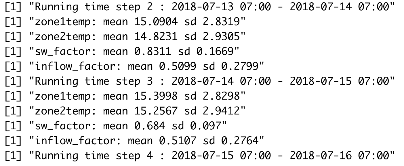
Your console will show a lot of messages from R that are mostly associated with reading and writing files. You will know that you simulation has started to work when you see the timestep being printed out to the console. This step will take a while.

Once the simulation is complete you will find a PDF and a netcdf (.nc) file in flare_simulation directory. The PDF is the plotted output and the netcdf file is the FLARE output.

4: Examining FLARE output

First, you can view the PDF that is output automatically. The PDF includes the mean and 95% CI for all depths simulated. The observations are added if they are available. If parameters are fit in the EnKF, they are also shown.

Example of FLARE output

Second, the netcdf output FLARE can be analyzed. Netcdf files are binary so you can not open them without special software. R has useful functions for working with netcdf files. For example, this is how you would analyze the mean temperature output from FLARE.

nc_file <- "example_output/test_H_2018_07_12_2018_07_15_F_16_4302020_15_13.nc"
nc <- nc_open(nc_file)

The data is stored as follows

print(nc)

## File example_output/test_H_2018_07_12_2018_07_15_F_16_4302020_15_13.nc (NC_FORMAT_NETCDF4):
## 
##      21 variables (excluding dimension variables):
##         float temp[time,ens,z]   (Contiguous storage)  
##             units: deg_C
##             _FillValue: 1.00000003318135e+32
##             long_name: temperature
##         float temp_mean[time,z]   (Contiguous storage)  
##             units: deg_C
##             _FillValue: 1.00000003318135e+32
##             long_name: temperature_mean
##         float temp_upperCI[time,z]   (Contiguous storage)  
##             units: deg_C
##             _FillValue: 1.00000003318135e+32
##             long_name: temperature_upperCI
##         float temp_lowerCI[time,z]   (Contiguous storage)  
##             units: deg_C
##             _FillValue: 1.00000003318135e+32
##             long_name: temperature_lowerCI
##         float qt_restart[states_aug,states_aug]   (Contiguous storage)  
##             units: -
##             _FillValue: 1.00000003318135e+32
##             long_name: restart covariance matrix
##         float x_restart[ens,states_aug]   (Contiguous storage)  
##             units: -
##             _FillValue: 1.00000003318135e+32
##             long_name: matrix for restarting EnKF
##         float x_prior[time,ens,states_aug]   (Contiguous storage)  
##             units: -
##             _FillValue: 1.00000003318135e+32
##             long_name: Predicted states prior to Kalman correction
##         float obs[time,obs_dim]   (Contiguous storage)  
##             units: various
##             _FillValue: 1.00000003318135e+32
##             long_name: temperature observations
##         int forecasted[time]   (Contiguous storage)  
##             units: -
##             _FillValue: -99
##             long_name: 0 = historical; 1 = forecasted
##         float surface_height_restart[ens]   (Contiguous storage)  
##             units: m
##             _FillValue: -99
##             long_name: Surface Height
##         float snow_ice_restart[ens,snow_ice_dim]   (Contiguous storage)  
##             units: m
##             _FillValue: -99
##             long_name: Snow (1), White Ice (2), Blue Ice (3)
##         float ice_thickness[time,ens]   (Contiguous storage)  
##             units: m
##             _FillValue: -99
##             long_name: Ice Thickness
##         float lake_depth[time,ens]   (Contiguous storage)  
##             units: m
##             _FillValue: -99
##             long_name: Depth of lake
##         float avg_surf_temp_restart[ens]   (Contiguous storage)  
##             units: deg_C
##             _FillValue: -99
##             long_name: Running Average of Surface Temperature
##         float running_residuals[qt_update_days,states]   (Contiguous storage)  
##             units: various
##             _FillValue: 1.00000003318135e+32
##             long_name: running residual for updating qt
##         float mixing_restart[ens,mixing_restart_vars_dim]   (Contiguous storage)  
##             units: various
##             _FillValue: 1.00000003318135e+32
##             long_name: variables required to restart mixing
##         float depths_restart[ens,depth_restart_vars_dim]   (Contiguous storage)  
##             units: various
##             _FillValue: 1.00000003318135e+32
##             long_name: depths simulated by glm that are required to restart 
##         float zone1temp[time,ens]   (Contiguous storage)  
##             units: deg_C
##             _FillValue: 1.00000003318135e+32
##         float zone2temp[time,ens]   (Contiguous storage)  
##             units: deg_C
##             _FillValue: 1.00000003318135e+32
##         float sw_factor[time,ens]   (Contiguous storage)  
##             units: -
##             _FillValue: 1.00000003318135e+32
##         float inflow_factor[time,ens]   (Contiguous storage)  
##             units: -
##             _FillValue: 1.00000003318135e+32
## 
##      10 dimensions:
##         time  Size:20
##             units: seconds
##             long_name: seconds since 1970-01-01 00:00.00 UTC
##         ens  Size:210
##             long_name: ensemble member
##         z  Size:28
##             units: meters
##             long_name: Depth from surface
##         states_aug  Size:32
##             long_name: length of model states plus parameters
##         obs_dim  Size:28
##             long_name: length of 
##         snow_ice_dim  Size:3
##             long_name: snow ice dims
##         qt_update_days  Size:30
##             long_name: Number of running days that qt smooths over
##         states  Size:28
##             long_name: states
##         mixing_restart_vars_dim  Size:17
##             long_name: number of mixing restart variables
##         depth_restart_vars_dim  Size:500
##             long_name: number of possible depths that are simulated in GLM
## 
##     6 global attributes:
##         title: Falling Creek Reservoir forecast
##         institution: Virginia Tech
##         GLM_version: GLM 3.0.0beta10
##         FLARE_version: v1.0_beta.1
##         time_zone_of_simulation: EST
##         forecast_issue_time: 2020-04-30 15:13:55

The key to understanding the file is the dimensions. For the variable temp_mean the first dimension is time and the second is z, which is depth. The actual values for these dimensions are in the variables with in the dimensions called time and z. The other key dimension is ens, which is the ensemble member. It is not present in temp_mean because that output variable is summarized across ensemble members.

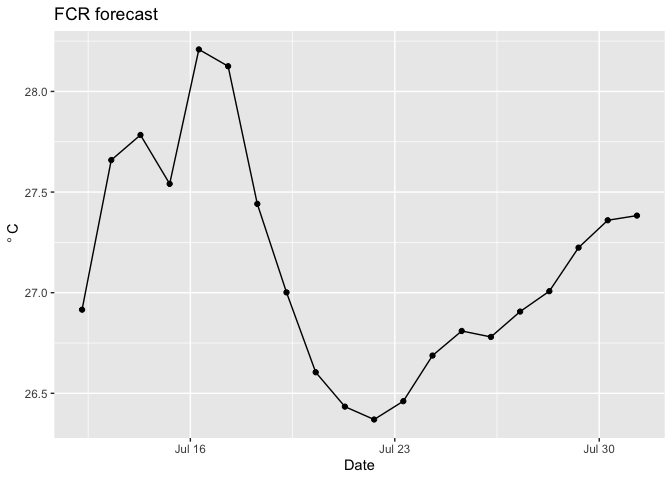
Plotting FLARE output

To visualize the output, you can use the following code

temp_mean <- ncvar_get(nc, varid = "temp_mean") #get the mean temperatures from the netcdf file
t <- ncvar_get(nc, varid = "time") #get the corresponding times from the netcdf file
t <- as.POSIXct(t, origin = '1970-01-01 00:00.00 UTC', tz = "EST") #format times as datetime
depths <- ncvar_get(nc, varid = "z")

focal_depth <- 1 #What depth are you interested in (meters)
depth_index <- which.min(abs(depths - 1))

d <- tibble(time = t, #create a dataframe of times and temperatures at the specified depth
            temp_mean = temp_mean[,depth_index])

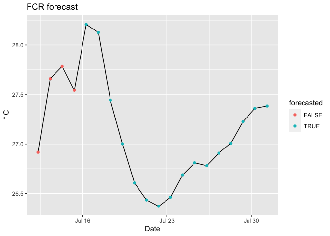
ggplot(d, aes(x = time, y = temp_mean)) + #plot mean temperature (modeled) at this depth over time
  geom_line() +
  geom_point() +
  labs(x = "Date", y = expression(~degree~C), title = "FCR forecast")

However, you do not know which points were based on observed drivers and data assimilation and which points were forecasted. To find the points that are forecasted you need the forecasted variable in the output.

forecasted <- ncvar_get(nc, varid = "forecasted") #binary. 1: forecasted, 0: not forecasted

focal_depth <- 1 #What depth are you interested in (meters)
depth_index <- which.min(abs(depths - 1))

d <- tibble(time = t, 
            temp_mean = temp_mean[,depth_index],
            forecasted = as.logical(forecasted))

ggplot(d) +
  geom_line(aes(x = time, y = temp_mean)) +
  geom_point(aes(x = time, y = temp_mean, color = forecasted))  +
  labs(x = "Date", y = expression(~degree~C), title = "FCR forecast")

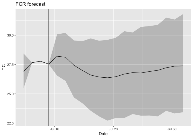
You can add the uncertainty using the following.

temp_mean <- ncvar_get(nc, varid = "temp_mean")
temp_upper95 <- ncvar_get(nc, varid = "temp_upperCI")
temp_lower95 <- ncvar_get(nc, varid = "temp_lowerCI")
forecasted <- ncvar_get(nc, varid = "forecasted")
t <- ncvar_get(nc, varid = "time")
depths <- ncvar_get(nc, varid = "z")
t <- as.POSIXct(t, origin = '1970-01-01 00:00.00 UTC', tz = "EST")

focal_depth <- 1 #What depth are you interested in (meters)
depth_index <- which.min(abs(depths - 1))

d <- tibble(time = t,
            temp_mean = temp_mean[,depth_index],
            temp_upper95 = temp_upper95[,depth_index],
            temp_lower95 = temp_lower95[,depth_index],
            forecasted = as.logical(forecasted))

ggplot(d,aes(x = time)) +
  geom_line(aes(y = temp_mean)) +
  geom_ribbon(aes(ymin = temp_lower95, ymax = temp_upper95), alpha = 0.25) +
  geom_vline(xintercept = last(d$time[which(d$forecasted == 0)])) + #vertical line marking the day of the forecast
  labs(x = "Date", y = expression(~degree~C), title = "FCR forecast")

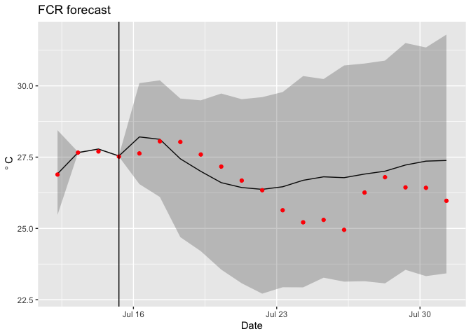
You can add observations

temp_mean <- ncvar_get(nc, varid = "temp_mean")
temp_upper95 <- ncvar_get(nc, varid = "temp_upperCI")
temp_lower95 <- ncvar_get(nc, varid = "temp_lowerCI")
forecasted <- ncvar_get(nc, varid = "forecasted")
t <- ncvar_get(nc, varid = "time")
depths <- ncvar_get(nc, varid = "z")
t <- as.POSIXct(t, origin = '1970-01-01 00:00.00 UTC', tz = "EST")
obs <- ncvar_get(nc, varid = "obs")

focal_depth <- 1 #What depth are you interested in (meters)
depth_index <- which.min(abs(depths - 1))

d <- tibble(time = t,
            temp_mean = temp_mean[,depth_index],
            temp_upper95 = temp_upper95[,depth_index],
            temp_lower95 = temp_lower95[,depth_index],
            forecasted = as.logical(forecasted),
            obs = obs[, depth_index])

ggplot(d,aes(x = time)) +
  geom_line(aes(y = temp_mean)) +
  geom_ribbon(aes(ymin = temp_lower95, ymax = temp_upper95), alpha = 0.25) +
  geom_point(aes(y = obs), color = "red") +
  geom_vline(xintercept = last(d$time[which(d$forecasted == 0)])) +
  labs(x = "Date", y = expression(~degree~C), title = "FCR forecast")

Finally, you can calculate the statistics of the forecast directly from the ensembles (rather than using the statistics already calculated in the netcdf file; these should be identical for mean and 95% confidence intervals)

temp <- ncvar_get(nc, varid = "temp")
forecasted <- ncvar_get(nc, varid = "forecasted")
t <- ncvar_get(nc, varid = "time")
t <- as.POSIXct(t, origin = '1970-01-01 00:00.00 UTC', tz = "EST")
depths <- ncvar_get(nc, varid = "z")
obs <- ncvar_get(nc, varid = "obs")

focal_depth <- 1 #What depth are you interested in (meters)
depth_index <- which.min(abs(depths - 1))

temp_lower95 <- rep(NA, length(t))
temp_upper95 <- rep(NA, length(t))
temp_mean <- rep(NA, length(t))
for(i in 1:length(t)){
  temp_lower95[i] <- quantile(temp[i, , depth_index],0.025) #calculate the 95% confidence interval from all ensemble members at each date
  temp_upper95[i] <- quantile(temp[i, , depth_index],0.975)
  temp_mean[i] <- mean(temp[i, , depth_index]) #calculate the mean of all ensemble members at each date
}

d <- tibble(time = t,
            temp_mean = temp_mean,
            temp_upper95 = temp_upper95,
            temp_lower95 = temp_lower95,
            forecasted = as.logical(forecasted),
            obs = obs[, depth_index])

d

## # A tibble: 20 x 6
##    time                temp_mean temp_upper95 temp_lower95 forecasted   obs
##    <dttm>                  <dbl>        <dbl>        <dbl> <lgl>      <dbl>
##  1 2018-07-12 07:00:00      26.9         28.4         25.5 FALSE       26.9
##  2 2018-07-13 07:00:00      27.7         27.7         27.6 FALSE       27.7
##  3 2018-07-14 07:00:00      27.8         27.8         27.8 FALSE       27.7
##  4 2018-07-15 07:00:00      27.5         27.6         27.5 FALSE       27.5
##  5 2018-07-16 07:00:00      28.2         30.1         26.6 TRUE        27.6
##  6 2018-07-17 07:00:00      28.1         30.2         26.1 TRUE        28.1
##  7 2018-07-18 07:00:00      27.4         29.6         24.7 TRUE        28.0
##  8 2018-07-19 07:00:00      27.0         29.5         24.2 TRUE        27.6
##  9 2018-07-20 07:00:00      26.6         29.7         23.6 TRUE        27.2
## 10 2018-07-21 07:00:00      26.4         29.5         23.1 TRUE        26.7
## 11 2018-07-22 07:00:00      26.4         29.6         22.7 TRUE        26.3
## 12 2018-07-23 07:00:00      26.5         29.8         22.9 TRUE        25.6
## 13 2018-07-24 07:00:00      26.7         30.3         22.9 TRUE        25.2
## 14 2018-07-25 07:00:00      26.8         30.2         23.3 TRUE        25.3
## 15 2018-07-26 07:00:00      26.8         30.7         23.1 TRUE        24.9
## 16 2018-07-27 07:00:00      26.9         30.8         23.1 TRUE        26.3
## 17 2018-07-28 07:00:00      27.0         30.9         23.1 TRUE        26.8
## 18 2018-07-29 07:00:00      27.2         31.5         23.5 TRUE        26.4
## 19 2018-07-30 07:00:00      27.4         31.3         23.3 TRUE        26.4
## 20 2018-07-31 07:00:00      27.4         31.8         23.4 TRUE        26.0

5: Running GLM-AED

To run GLM-AED fist copy a glm namelist file to your simulation flare_simulation directory. Thre are two example options in the FLARE/example_configuration_files directory. They differ in whether they include an additional inflow and outflow that represents the SSS (bottom-water oxygenation system).

• glm3_wAED_wSSS.nml: Include the SSS inflows and outflows
• glm3_wAED_woSSS.nml: Excludes the SSS inflows and outflows

Second, copy an aed namelist file to your simulation flare_simulation directory. Thre are two example options in the FLARE/example_configuration_files directory. They differ in whether they include all the water quality variables in AED or only oxygen.

• aed2.nml: All variables
• aed2_only_Oxy.nml: Only oxygen

Third, modify the following in configure_FLARE.R:

• include_wq: Set to TRUE
• base_GLM_nml: full path to the glm namelist matches the one in your flare_simulation that includes AED.
• base_AED_nml: full path to your aed namelist
• base_AED_phyto_pars_nml: full path to your phyto_pars namelist
• base_AED_zoop_pars_nml: full path to your zoop_pars namelist

Finally, confirm that the following varibles in configure_FALRE.R match your desire use of the data:

• do_methods: these are the names of the different measurement methods as defined in the temp_oxy_chla_qaqc.R and extract_CTD.R scripts
  • current values for FCR: exo, do, ctd
• chla_methods: these are the names of the different measurement methods as defined in the temp_oxy_chla_qaqc.R and extract_CTD.R scripts
  • current values for FCR: exo, ctd
• fdom_methods: these are the names of the different measurement methods as defined in the temp_oxy_chla_qaqc.R and extract_nutrients.R scripts
  • current values for FCR: exo, grap_sample
• nh4_methods: these are the names of the different measurement methods as defined in the extract_nutrients.R
  • current values for FCR: grap_sample
• no3_methods: these are the names of the different measurement methods as defined in the extract_nutrients.R
  • current values for FCR: grap_sample
• srp_methods: these are the names of the different measurement methods as defined in the extract_nutrients.R
• time_threshold_seconds_oxygen: this is the number of seconds that an observation has to be within the start_time_local to be used in the analysis
• time_threshold_seconds_chla: this is the number of seconds that an observation has to be within the start_time_local to be used in the analysis
• time_threshold_seconds_fdom: this is the number of seconds that an observation has to be within the start_time_local to be used in the analysis
• time_threshold_seconds_nh4: this is the number of seconds that an observation has to be within the start_time_local to be used in the analysis
• time_threshold_seconds_no3: this is the number of seconds that an observation has to be within the start_time_local to be used in the analysis
• time_threshold_seconds_srp: this is the number of seconds that an observation has to be within the start_time_local to be used in the analysis

6: Modifying FLARE

Turning off data assimilation

• Our for modification to FLARE will be remove a source of uncertainty in the forecast The uncert_mode allows you to do this easily based on the following:
  • 1 = all types
  • 2 = no uncertainty
  • 3 = only process uncertainty
  • 4 = only NOAA weather forecast uncertainty
  • 5 = only initial condition uncertainty
  • 6 = only initial condition uncertainty and no state updating with EnKF
  • 7 = only parameter uncertainty
  • 8 = only meteorology downscaling uncertainty
  • 9 = no sources of uncertainty and no state updating with EnKF
  • 11 = all sources of uncertainty and no state updating with EnKF

In this tutorial, explore how data assimilation influences your forecast. To do this modify the following two variables and source the code:

• uncert_mode <- 11 (in configure_FLARE.R)
• sim_name <- "NO_DA" (in initiate_forecast_example.R)
• source initiate_forecast_example.R

Removing parameter estimation

You can remove the parameter optimization so that FLARE only uses data assimilation to update the initial conditions of a forecast. * In configure_FLARE.R add the following code to line 250. These remove the parameters from EnKF.

par_names <<- c()
par_names_save <<- c()
par_nml <<- c()
par_init_mean <<- c()
par_init_lowerbound <<- c()
par_init_upperbound <<- c()
par_lowerbound <<- c()
par_upperbound <<- c()
par_init_qt <<- c()
par_units <<- c()

Increasing observational uncertainty

The second modification you will do is to to increase the observational uncertainty. In configure_FLARE.R set obs_error_temperature_intercept = 1. Then Source initiate_forecast_example.R. Importantly, observational uncertainty is in variance units (the square of standard deviation).

Observational uncertainty has two components.

• obs_error_temperature_intercept: the component that is independent of the measurement magnitude
• obs_error_temperature_slope: the component that linearly scales with the magnitude of the measurement

Changing the ensemble size

The variable ensemble_size allows you to adjust the size of the ensemble. You can use any value if you are using data assimilation with observed drivers. If you are forecasting then ensemble_size must be a multiple of 21 * n_ds_members, where 21 is the number of NOAA GEF ensemble members.

Changing the number of depths simulated

The variable modeled_depths allows you to adjust the depths that FLARE simulates

7: Modifying FLARE for a new lake

We are in the process of making it easier to apply FLARE to a new lake. Currently applying FLARE to a new lake requires modifying R scripts because data streams (meteorology, inflow, and in situ data) formats differ between lakes. The following steps are required to set up a new lake:

Modify the glm namelist

Within the glm namelist (glm3_woAED.nml in the tutorial), at minimum you need to change the variables in the &morphometry, &inflow, and &outflow sections. Please see the GLM users guide for more information about the variables in these sections of the namelist. Additionally, the paper describing GLM 3.0.0 describes variables in the namelist

You will also need to modify the zone_heights in the &sediment section for your new lake. Currently, FLARE only handles two zone_heights, where the first value is the top depth of the bottom layer and the second value is the top of the top layer (the maximum depth of the lake).

Other variables to modify are:

• Kw: the light extension coefficient

The FLARE code automatically updates all the variables in &init_profiles

Modify Configure_flare.R

Within configure_flare.R you will need to update:

• lake_name: this is the code for the lake. It must match the the lake specific directory within your /FLARE/Rscripts/[lake_name] directory.
• lake_latitude: Degrees North
• lake_longitude: Degrees West
• local_tzone : Standard time, a time zone that R understands
• lake_depth_init: Initial depth of the lake
• modeled_depths: depths that are simulated

You will also need to update the file names for the driver and in situ data:

• insitu_obs_fname: the in situ data (temperature, do, etc)
• met_obs_fname: the meteorological station
• inflow_file1: the first inflow (the weir at FCR)
• inflow_file2: an optional second inflow
• outflow_file1: an optional outflow (NOTE: this currently is not used in FLARE)

FLARE also allows you to include a separate file for CTD depth profiles:

• ctd_fname: a value of NA is needed if you do not have or do not want to use CTD measurements

Importantly, insitu_obs_fname, met_obs_fname, and inflow_file1 require two file names. The first is the realtime file that has not had QAQC applied (i.e,just downloaded from the sensor). The second is file that has QAQC applied (i.e, a file from a data repository). If any time periods overlap between the two files, FLARE will default the second (QAQCed) file. Historical data assimilation applications will use the QAQCed file. If you are missing one of the two file, the vector should have an NA in its place.

You will need to specify how to process data files:

• temp_methods: these are the names of the different measurement methods used to aquire data (e.g. CTD profile, in situ thermistor), as defined in the temp_oxy_chla_qaqc.R and, potentially, extract_CTD.R, scripts that you have modified for the new lake.
  • current values for FCR: thermistor, exo, do, ctd
• time_threshold_seconds_temp: this is how close a measurement needs to be to the forecast time (start_time_local) to be used in the analysis, in seconds.
• distance_threshold_meter: this is the distances in meters that an observation has to be within to be matched to a value in modeled_depths.

Finally there are some plotting configurations:

• focal_depths_manager: the depths that are included in the plot with the % chance of turnover
• turnover_index_1: the top depth used in the calculation of whether the lake is mixed
• turnover_index_2: the bottom depth used in the calculation of whether the lake is mixed

Creating and modifying a lake-specific Rscripts directory

You need to create a /FLARE/Rscripts/[lake_name] directory and move all the files in /FLARE/Rscripts/fcre to that directory.

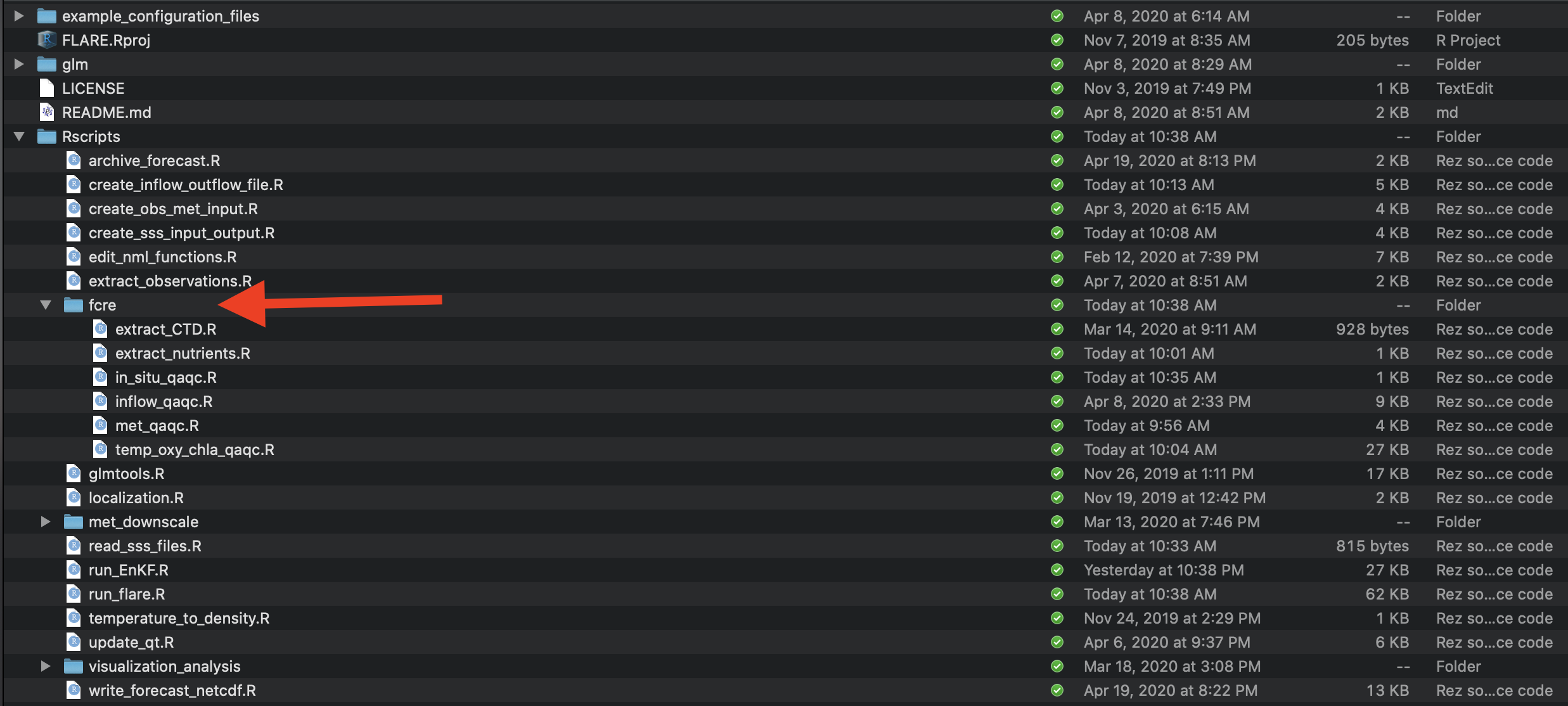
You may need to modify the following files that you moved to /FLARE/Rscripts/[lake_name], depending on how similar your data file formats are to the files used at fcre.

• met_qaqc.R:
  • Inputs:
    • fname
    • cleaned_met_file
    • input_file_tz
    • local_tzone
    • full_time_local
  • Outputs: needs to write a csv file with the following columns
    • timestamp
    • ShortWave
    • LongWave
    • AirTemp
    • RelHum
    • WindSpeed
    • Rain
• inflow_qaqc.R:
  • Inputs:
    • realtime_file
    • qaqc_file
    • nutrients_file
    • cleaned_inflow_file
    • local_tzone
    • input_file_tz
  • Output: needs to write a csv file with the following columns
    • GLM only: time, FLOW, TEMP, SALT
    • GLM AED: variables defined in wq_names (configure_FLARE.R)
• in_situ_qaqc.R: This function calls the following functions that need to be modified based on the format of the lake data streams
  • Inputs:
    • insitu_obs_fname
    • data_location
    • maintenance_file
    • ctd_fname
    • nutrients_fname
    • cleaned_observations_file_long
    • lake_name
    • code_folder
  • Outputs: needs to write a csv file with the following columns
    • timestamp: date-time class
    • depth: meters
    • variable: measurement variable
    • method: user defined string defining the type of measurement. Matches methods in configure_FLARE.R (i.e., temp_methods)
  • in_situ_qaqc.R calls the following functions
    • temp_oxy_chla_qaqc.R:
      • Inputs:
        • realtime_file
        • qaqc_file
        • maintenance_file
        • input_file_tz
      • Output: data frame with the following columns
        • timestamp: date-time class
        • depth: meters
        • variable: measurement variable
        • method: user defined string defining the type of measurement. Matches methods in configure_FLARE.R (i.e., temp_methods)
    • extract_CTD.R:
      • Inputs:
        • fname
        • input_file_tz
        • local_tzone
      • Output: data frame with the following columns
        • timestamp: date-time class
        • depth: meters
        • variable: measurement variable
        • method: user defined string defining the type of measurement. Matches methods in configure_FLARE.R (i.e., temp_methods)
    • extract_nutrients.R:
      • Inputs:
        • fname
        • input_file_tz
        • local_tzone
      • Output: data frame with the following columns
        • timestamp: date-time class
        • depth: meters
        • variable: measurement variable
        • method: user defined string defining the type of measurement. Matches methods in configure_FLARE.R (i.e., temp_methods)

Appendix: FLARE Configurations

A guide to the variables in configure_flare.R

General set-up

• GLMversion: string of GLM version
• FLAREversion: string of FLARE version
• use_null_model: Whether to use the persistance null model or GLM
  • TRUE: use persistance null model
  • FALSE: use GLM
• include_wq: Whether to use GLM-AED or just GLM
  • TRUE: use GLM-AED
  • FALSE: only use GLM
• uncert_mode: code for the type of uncertainty to include in simulation
  • 1 = all types of uncertainty
  • 2 = no uncertainty
  • 3 = only process uncertainty
  • 4 = only NOAA weather forecast uncertainty
  • 5 = only initial condition uncertainty
  • 6 = only initial condition uncertainty and no state updating with the EnKF
  • 7 = only parameter uncertainty
  • 8 = only meteorology downscaling uncertainty
  • 9 = no sources of uncertainty and no state updating with EnKF
  • 11 = all sources of uncertainty and no state updating with EnKF
• single_run: Removes uncertainty and only simulates 3 ensemble members
  • TRUE:: only simulates 3 ensemble members without uncertainty
  • FALSE: all ensemble members and uncertainty specified in uncert_mode
• pull_from_git: Flag to pull data from GitHub
  • TRUE: Pull
  • FALSE: Don’t pull (needed if you are offline)
• push_to_git: Push results to GitHub
  • TRUE: Push
  • FALSE: Don’t Push (needed if you are offline)

Lake specific variables

• lake_name: four letter code name for lake. Match lake directy in FLARE/Rscripts and in the NOAA GEF files
• lake_latitude: Degrees North
• lake_longitude: Degrees West
• local_tzone: In standard time. Must be recognized by R.

Weather forcing options

• use_future_met
  • TRUE: use NOAA forecast for “Future”
  • FALSE = use observed weather for “Future”; only works if “forecasting” past dates
• DOWNSCALE_MET: apply spatial and temporal downscaling
  • TRUE: downscale
  • FALSE: don’t downscale
• noaa_location: full path of directory with NOAA GEF files
  • paste0(data_location, “/”,lake_name,“/”)
• downscaling_coeff: full path to the Rdata that has previously estimated downscaling coefficients
  • paste0(data_location, “/manual-data/debiased.coefficients.2018_07_12_2019_07_11.RData”)
  • NA: no previous coefficient, calculate within simulation if DOWNSCALE_MET == TRUE.
• met_ds_obs_start: Starting date to include in estimation of downscaling coefficients
  • date class (as.Date("2019-07-11"))
• met_ds_obs_end: Ending date to include in estimation of downscaling coefficients
  • date class (as.Date("2019-07-11"))
• missing_met_data_threshold: PENDING

Inflow options

• use_future_inflow: Use forecast inflow vs. observed inflow (if available)
  • TRUE: Future inflow
  • FALSE: Observed inflow
• future_inflow_flow_coeff: Vector of three numbers
  • Intercept
  • Coefficient with lagged flow rate
  • Coefficient with lagged rain
• future_inflow_flow_error: Standard deviation of future flow model
• future_inflow_temp_coeff:
  • Intercept
  • Coefficient with lagged water temperature
  • Coefficient with lagged air temperature
• future_inflow_temp_error: Standard deviation of future temperature model

GLM namelist files

• base_GLM_nml: full path to the glm namelist
  • example: paste0(forecast_location,“/glm3_woAED.nml” )
• base_AED_nml: full path to the aed namelist
• base_AED_phyto_pars_nml: full path to the phyto_pars namelist
• base_AED_zoop_pars_nml: full path to the zoop_pars namelist

Depth information

• modeled_depths: Vector of depths are that represented in the EnKF

Ensemble description

• ensemble_size: Total number of ensemble members
• n_ds_members: Number of random samples drawn from each NOAA GEF ensemble member based on the variance-covariance matrix from downscaling analysis.
• n_inflow_outflow_members: Number of random samples drawn from the normal distribution describing the residual error in the inflow rate and inflow temperature model

Process uncertainty adaption

• use_cov: Allow for covariance of process uncertainty across depths
  • TRUE: Include
  • FALSE: Don’t include
• adapt_qt_method:
  • 0 = no adapt,
  • 1 = variance in residuals
• num_adapt_days: Number of days included in generation of the variance- covariance matrix of the residuals. The matrix represents process uncertainties.
• Inflat_pars: The variance inflation factor applied to the parameter component of the ensemble. Value greater than 1.

Parameter calibration information

• par_names: vector of GLM names of parameter values estimated
• par_names_save: vector of names of parameter values estimated that are desired in output and plots
• par_nml: vector of nml file names that contains the parameter that is being estimated
• par_init_mean: vector of initial mean value for parameters
• par_init_lowerbound: vector of lower bound for the initial uniform distribution of the parameters
• par_init_upperbound: vector of upper bound for the initial uniform distribution of the parameters
• par_lowerbound: vector of lower bounds that a parameter can have
• par_upperbound: vector of upper bounds that a parameter can have
• par_init_qt: Not used
• par_units: Units of parameter for plotting

Observation information

• realtime_insitu_location: full path to the directory with the non-QAQCed in situ data (i.e., thermistor chain)

• realtime_met_station_location: full path to the directory with the non-QAQCed met station data

• manual_data_location: full path to the directory with the QAQCed datasets

• realtime_inflow_data_location: full path to the directory with the non-QAQCed inflow data.

• ctd_fname: full path of CTD file

• nutrients_fname: full path of nutrients file

• insitu_obs_fname: vector of two full paths

  • 1: path of the realtime file (required)
  • 2: path of respository (QAQCed) file (if not used, must have NA)

• variable_obsevation_depths: Use the depth measurement from the exo sonde (on a buoy; constant depth from surface) to convert the depths of a fixed thermistor chain to distance from surface

  • TRUE: convert
  • FALSE: don’t convert

• ctd_2_exo_chla: slope and intercept of linear regression that converts chla values from the CTD to values from the exo sonde

• met_obs_fname: vector of two full paths

  • 1: path of the realtime file (required)
  • 2: path of respository (QAQCed) file (if not used, must have NA)

• inflow_file1: vector of two full paths

  • 1: path of the realtime file (required)
  • 2: path of respository (QAQCed) file (if not used, must have NA)

• outflow_file1: Not current used

• inflow_file2: Not current used

• temp_methods: these are the names of the different measurement methods as defined in the temp_oxy_chla_qaqc.R and extract_CTD.R scripts

  • current values for FCR: thermistor, exo, do, ctd

• do_methods: these are the names of the different measurement methods as defined in the temp_oxy_chla_qaqc.R and extract_CTD.R scripts

  • current values for FCR: exo, do, ctd

• chla_methods: these are the names of the different measurement methods as defined in the temp_oxy_chla_qaqc.R and extract_CTD.R scripts

  • current values for FCR: exo, ctd

• fdom_methods: these are the names of the different measurement methods as defined in the temp_oxy_chla_qaqc.R and extract_nutrients.R scripts

  • current values for FCR: exo, grap_sample

• nh4_methods: these are the names of the different measurement methods as defined in the extract_nutrients.R

  • current values for FCR: grap_sample

• no3_methods: these are the names of the different measurement methods as defined in the extract_nutrients.R

  • current values for FCR: grap_sample

• srp_methods: these are the names of the different measurement methods as defined in the extract_nutrients.R

• time_threshold_seconds_temp: this is how close a measurement needs to be to the forecast time (start_time_local) to be used in the analysis, in seconds.

• time_threshold_seconds_oxygen: this is how close a measurement needs to be to the forecast time (start_time_local) to be used in the analysis, in seconds.

• time_threshold_seconds_chla: this is how close a measurement needs to be to the forecast time (start_time_local) to be used in the analysis, in seconds.

• time_threshold_seconds_fdom: this is how close a measurement needs to be to the forecast time (start_time_local) to be used in the analysis, in seconds.

• time_threshold_seconds_nh4: this is how close a measurement needs to be to the forecast time (start_time_local) to be used in the analysis, in seconds.

• time_threshold_seconds_no3: this is how close a measurement needs to be to the forecast time (start_time_local) to be used in the analysis, in seconds.

• time_threshold_seconds_srp: this is how close a measurement needs to be to the forecast time (start_time_local) to be used in the analysis, in seconds.

• distance_threshold_meter: this is the distances in meters that an observation has to be within to be matched to a value in modeled_depths.

Initial Conditions (GLM)

• lake_depth_init: initial lake depth (meters)
• default_temp_init: vector of initial temperature profile
• default_temp_init_depths: vector of depths in initial temperature profile
• the_sals_init: vector of initial salinty values
• default_snow_thickness_init: initial snow thickness (cm)
• default_white_ice_thickness_init: initial white ice thickness (cm)
• default_blue_ice_thickness_init: initial blue ice thickness (cm)

Water quality variable information

• tchla_components_vars: The names of the phytoplankton groups that contribute to total chl-a in GLM
• wq_names: GLM names of the water quality variables modeled. Not used if include_wq == FALSE
• biomass_to_chla: Carbon to chlorophyll ratio (mg C/mg chla) for each group in tchla_components_vars.
  • 12 g/ mole of C vs. X g/ mole of chla
• init_donc: Initial ratio of DON:DOC
• init_dopc: Initial ratio of DOP:DOC
• init_ponc: Initial ratio of PON:POC
• init_popc: Initial ratio of
• OXY_oxy_init: Initial concentration (mmol/m3)
• CAR_pH_init: Initial concentration (mmol/m3)
• CAR_dic_init: Initial concentration (mmol/m3)
• CAR_ch4_init: Initial concentration (mmol/m3)
• SIL_rsi_init: Initial concentration (mmol/m3)
• NIT_amm_init: Initial concentration (mmol/m3)
• NIT_nit_init: Initial concentration (mmol/m3)
• PHS_frp_init: Initial concentration (mmol/m3)
• OGM_doc_init: Initial concentration (mmol/m3)
• OGM_poc_init: Initial concentration (mmol/m3)
• OGM_pon_init: Initial concentration (mmol/m3)
• OGM_pop_init: Initial concentration (mmol/m3)
• NCS_ss1_init: Initial concentration (mmol/m3)
• PHS_frp_ads_init: Initial concentration (mmol/m3)
• PHY_TCHLA_init: Initial concentration (ug/L)
• init_phyto_proportion: vector of the initial proportion of total chla that is each phytoplankton group in tchla_components_vars represents. Must add up to 1.0

Observation uncertainty

• obs_error_temperature_intercept: the component that is independent of the measurement magnitude
• obs_error_temperature_slope: the component that linearly scales with the magnitude of the measurement
• obs_error_wq_intercept_phyto: Not used
• obs_error_wq_slope_phyto: Not used
• obs_error_wq_intercept: the component that is independent of the measurement magnitude. A vector of with the same length as wq_names
• obs_error_wq_slope: the component that linearly scales with the magnitude of the measurement. A vector of with the same length as wq_names

Process uncertainty

• temp_process_error: variance of process uncertainty
• OXY_oxy_process_error: variance of process uncertainty
• CAR_pH_process_error: variance of process uncertainty
• CAR_dic_process_error: variance of process uncertainty
• CAR_ch4_process_error: variance of process uncertainty
• SIL_rsi_process_error: variance of process uncertainty
• NIT_amm_process_error: variance of process uncertainty
• NIT_nit_process_error: variance of process uncertainty
• PHS_frp_process_error: variance of process uncertainty
• OGM_doc_process_error: variance of process uncertainty
• OGM_poc_process_error: variance of process uncertainty
• OGM_don_process_error: variance of process uncertainty
• OGM_pon_process_error: variance of process uncertainty
• OGM_dop_process_error: variance of process uncertainty
• OGM_pop_process_error: variance of process uncertainty
• NCS_ss1_process_error: variance of process uncertainty
• PHS_frp_ads_process_error: variance of process uncertainty
• PHY_TCHLA_process_error: variance of process uncertainty
• PHY_process_error: variance of process uncertainty

Initial condition uncertainty

• temp_init_error: variance of initial temperature
• OXY_oxy_init_error: variance of initial oxygen
• CAR_pH_init_error: variance of initial pH
• CAR_dic_init_error: variance of initial DIC
• CAR_ch4_init_error: variance of initial CH4
• SIL_rsi_init_error: variance of initial Silica
• NIT_amm_init_error: variance of initial Ammonium
• NIT_nit_init_error: variance of initial Nitrate
• PHS_frp_init_error: variance of initial Phosphorus
• OGM_doc_init_error: variance of initial DOC
• OGM_poc_init_error: variance of initial POC
• OGM_don_init_error: variance of initial DON
• OGM_pon_init_error: variance of initial PON
• OGM_dop_init_error: variance of initial DOP
• OGM_pop_init_error: variance of initial POP
• NCS_ss1_init_error: variance of initial SS1
• PHS_frp_ads_init_error: variance of initial Adsorped Phosphorus
• PHY_TCHLA_init_error: variance of initial Total Chl-a
• PHY_init_error: variance of initial Phytoplankton biomass

Management specific variables

• simulate_SSS: include SSS (bottom-water oxygenation) in simulations with observed drivers (i.e., data assimilation simulations)
  • TRUE: include
  • FALSE: don’t include
• forecast_no_SSS: Include SSS in forecast
  • TRUE: include
  • FALSE: don’t include
• use_specified_sss: Use sss inflow and oxygen from file in forecast. If FALSE then provide forecast_SSS_flow and forecast_SSS_Oxy.
• forecast_SSS_flow: Flow rate of SSS in forecast (m3/day)
• forecast_SSS_Oxy: Oxygen concentration of SSS in forecast (mmol/m3)
• sss_fname: full path to the file that has the SSS Flow and oxygen data
• sss_inflow_factor: a scalar to multiply FLOW rate of SSS
• sss_depth: The depth (meters) of the SSS inflow/outflow

Plotting related options

• focal_depths_manager: A vector of depths that are included in the plot with the % change of turnover.
• turnover_index_1: the top depth used in the calculation of whether the lake is mixed
• turnover_index_2: the bottom depth used in the calculation of whether the lake is mixed